Visualizing Newton’s Method

Well for most of us winter break is coming to an end, or for the unlucky, might have already ended, which means its time to start thinking about teaching again. One of the topics commonly covered in a first or second semester of calculus is the use of Newton’s method to approximate roots of functions. Recall the basic approach of Newton’s method is that given a real valued differentiable function and an initial condition we let

$$x_n=x_{n-1}-\frac{f(x_{n-1})}{f’(x_{n-1})},$$

and then, under certain assumptions, should converge to a root of .

When I’ve taught Newton’s method, I tried to stress that this method is not guaranteed to always work and can be fairly sensitive to the initial condition . Going into the precise details of when the method will in fact work is well beyond my first semester calculus students. That said, I am not sure they’ve ever really appreciated these points. In fact, to be completely honest, I am not sure I completely appreciated some of the aspects of these things before I started teaching.

That said, one way to visualize some of these complexities is via a cool program called FractalStream. For example, using FractalStream, we can run the following script:

iterate z – (z^3 – 1)/(3*z^2) until z stops.

and then turn on autocoloring – under the color settings – and we get the following interesting picture of the complex plane colored red, blue, and green:

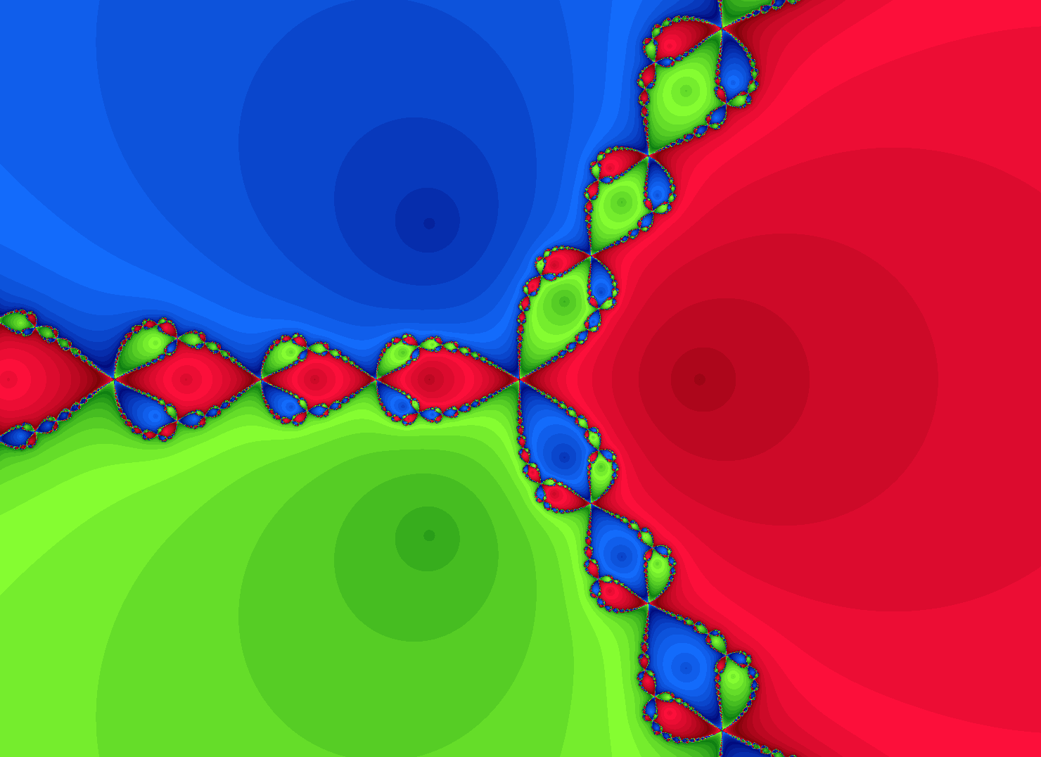
Newton’s method plot for z^3-1.

Given the above script, FractalStream takes each point in the complex plane and iterates it under the given map until the sequence seems to stops. It then colors that initial point depending on where the sequence of iterates ended. That is to say, since we chose to iterate the function:

$$N(z)=z-\frac{z^3-1}{3z^2}$$

the above script actually performs Newton’s method using the polynomial for each initial value and labels each value by which root we end at (assuming we end at a root).

In the above example, we see there are three colors since has three roots. Specifically green corresponds to the root 1, blue to , and finally red to the root . Notice that while there is a large area round each root in which Newton’s method converges quickly to that root the areas sort of between each root show more complex behavior. In particular, in this region we see just how sensitive to the initial condition Newton’s method becomes. Additionally, using the orbit tool in FractalStream we get a sense that points in this region take longer to converge:

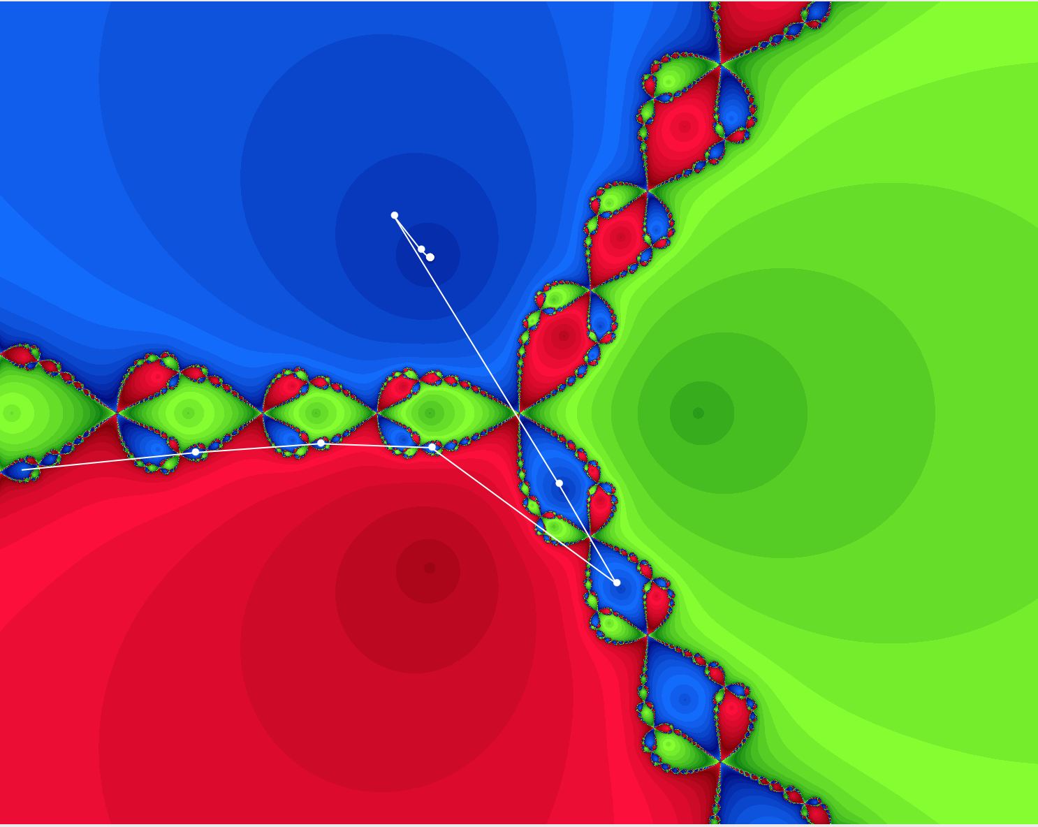
Forward iterates of a point converge to a root of z^3-1 under Newton’s method.

In this picture the white dot marks each forward iterate under the map of the point chosen.

We can create similar plots for other polynomials as well. For example, the plot for looks quite a bit different than the one for — in part because all the roots are real.

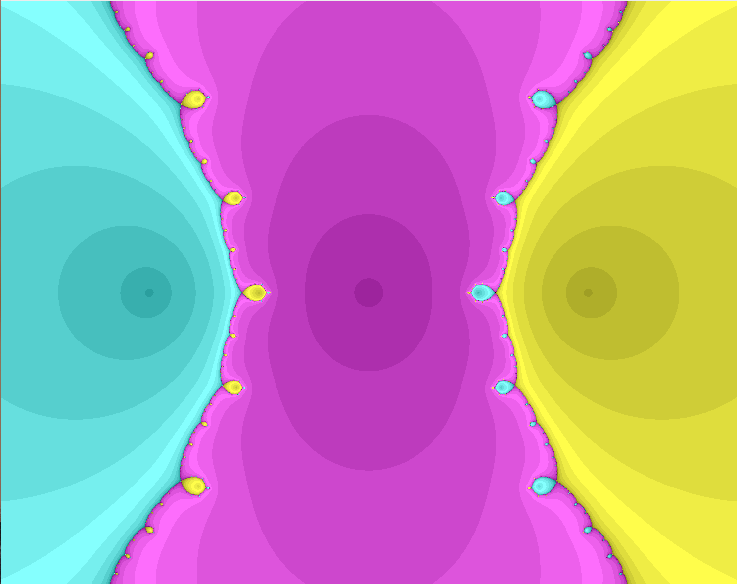
Newton’s method plot for z^3-3z.

It’s pretty fun just playing around with what plots various polynomials produce!

Why these pictures look the way they do has to do with complex dynamics, which is a really awesome subject. If you want to learn more about these pictures and what is going on you might want to check out either Dynamics in One Complex Variable by Milnor or Complex Dynamics by Carleson and Gamelin. However, even for those not interested in complex dynamics these pictures might be something fun to show your students next time you teach Newton’s method!