In posts 1-3 we were able to reduce all of the geometry of a curve in 3-space to an interval ![[a,b]\subset \mathbb{R}](https://s0.wp.com/latex.php?latex=%5Ba%2Cb%5D%5Csubset+%5Cmathbb%7BR%7D&bg=ffffff&fg=000&s=0&c=20201002) along with two or three real-valued functions. We also discussed when two sets of such data give equivalent (overlapping) curves. This enabled us to patch together a collection of such sets of data into one unified spatial curve.
along with two or three real-valued functions. We also discussed when two sets of such data give equivalent (overlapping) curves. This enabled us to patch together a collection of such sets of data into one unified spatial curve.
We then studied the specific example of re-defining the metric on the plane so that its geometry is precisely that of a 2-sphere. We saw that for measurements of angles, lengths, and areas, all we need is a dot-product on vectors. Given an open domain in the plane, once we have a dot-product, we will be able to make such measurements. Our goal in this post is to make the following definition of a manifold more tangible.
Begin with a topological space  . (Note we cannot talk about any structure other than continuous maps from or to this space.) Assume that for every
  , there is an open neighborhood
  of
of  homeomorphic to an open domain
  in the plane:
  These are called “charts”, or coordinate maps.
Given this the question now is: How do we make sense of the notions of  -ness and length for a curve
  ? One way we might hope to do this is by using our coordinate maps. That is we say that
  is if
is if  is C1C1 and we define the length of C to be the length of .
As illustrated in a picture in the previous post, this definition of -ness is not a satisfactory one because some curves will lie simultaneously in two neighborhoods, say and  , and there is no guarantee that if its image in is , it must also be in .
However, the two images are transformed to one another by the map 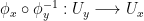 (See the previous article for the reason.) Therefore, if these “transition maps” between subsets of
  are , then without ambiguity, we can define a subset of to be a curve if its image under any (and hence all) of the chart maps is a curve in .
The space together with the data of coordinate charts with the properties above is a 2-dimensional manifold.
As sketched above, for such manifolds, it is meaningful to talk about curves, or functions  . In the latter case, we say
  is if
is if  is for all .
Hopefully, now, the idea is starting to make sense. A  manifold is a topological space with charts whose transition maps are . For these manifolds, we can talk about second derivative of functions. A smooth manifold is one with smooth, i.e.
  , transition maps… Well, as is noted in [1, pg. 9], “Usually additional technical assumptions on the topological space are made to exclude pathological cases. It is customary to require that the space be Hausdorff and second countable.”
Definition: “A  n-manifold” is a Hausdorff and second countable topological space, with charts that map into open domains of
  such that the transition maps are .
Where did the metric go?! How do we measure lengths?
Remember I said we might try to define the length of a curve  by saying it is equal to the length of the curve lying in ? Well, this begs the question: How do we compute the length of , because might have a metric other than the usual Euclidean one. For example, recall the metric on the plane from our example in the fourth post in this series. This means we run into a problem similar to the one we had when defining -ness. If each has its own metric, then a curve on the manifold may have different lengths, depending on the chart we use for the measurement. This will make the length undefinable by looking at charts, unless, some very intricate compatibility assumptions are imposed on the metrics of the ‘s.
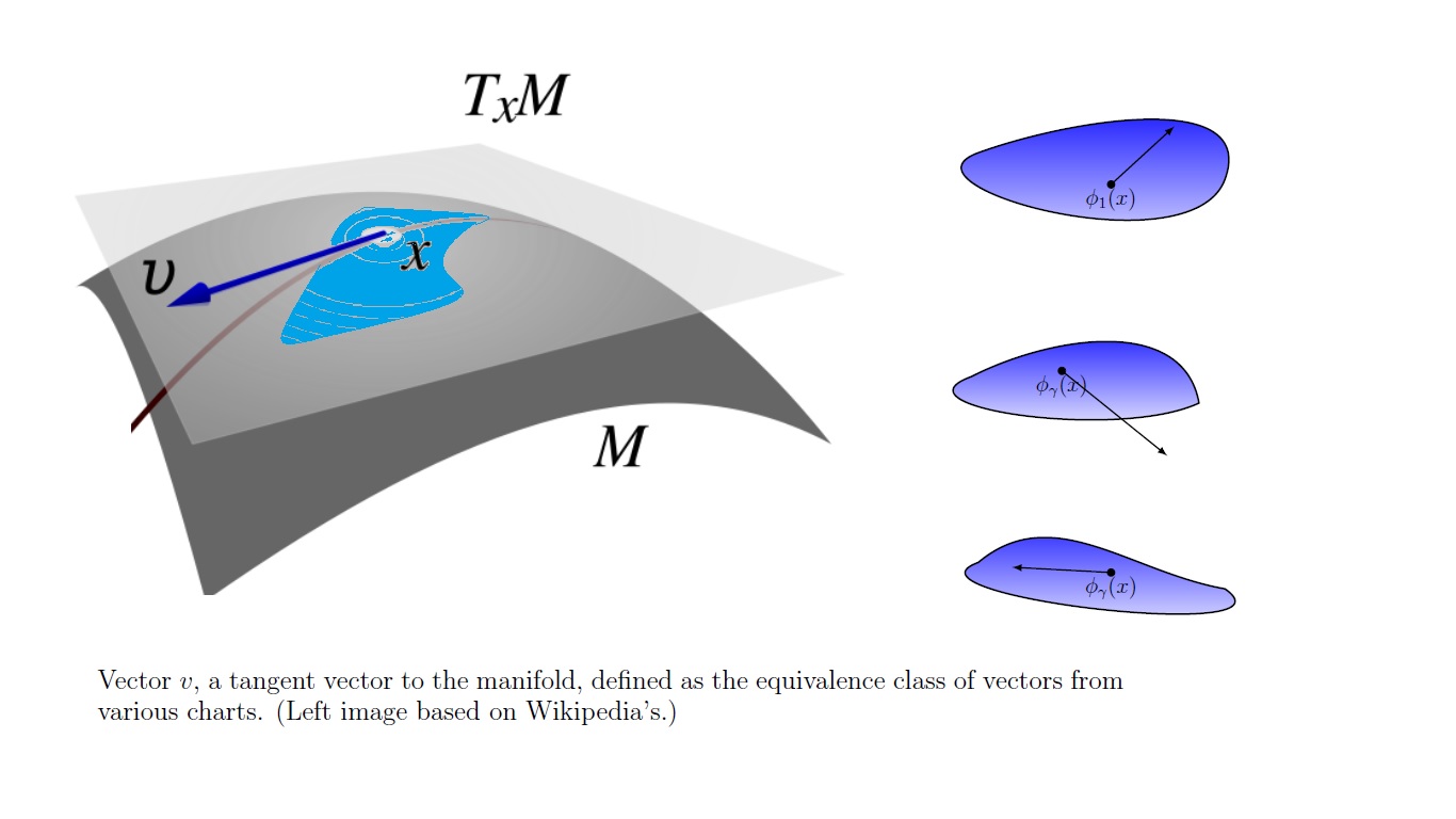
The good news is that one usually takes a different approach: A metric is built on the manifold upfront, rather than pieced together from collection of metrics on various ‘s that happen to magically be compatible in an complex manner. The key thing that makes this direct construction on the metric on a manifold possible, is the existence of “the tangent space”.
Fix a point , a manifold. In a chart  , the point is represented by
  . Since
  is bijective and , its derivative at the point existences, and is a
  invertible matrix, mapping vectors centered at to vectors centered at
  Thus, if we fix a vector
  at , then in any other chart
  there is a corresponding vector
  centered at
  . We call this collection of vectors, one from each chart, “a tangent vector to at .” By varying in
  , we see that the collection of all tangent vectors to at is in one-to-one relation with the vector space of all vectors centered at
  , which in turn is a copy of the vector space
  Thus, this collection is naturally a vector space. We denote it by
  . The key feature is that the tangent spaces were constructed from charts and not from an ambient space in which sits in.

Definition: “A metric” on is a choice of an inner product on each of the tangent spaces that continuously depends on .
In our example of the plane with the metric of a sphere, attached at each  , we think of a copy of the vector space . Then the inner product of the plane centered at is
  times the usual inner product of the plane.
What happens is that for the low dimensional tangible cases where we have a hyper-surface in a Euclidean space this abstract notion of a tangent space coincides with the “tangent plane” to the surface. For example, the tangent space to the sphere in  is the copy of 2-plane touching the sphere at one point. The vectors in this tangent can be alternatively viewed as vectors in , and therefore, their inner product is defined. Therefore, by “cheating”, most visualizable spaces come with an inner product. (This is, of course, far from being the only one.) Notice we are cheating, because, we are not supposed to work with an ambient space. Here we look at the ambient space to come up with an inner product, and then forget about the ambient space again, thus, ending with a metric in the manifold sense.
Definition: A Riemannian manifold is a smooth manifold equipped with a smooth inner-product.
Riemannian manifolds are where we can do measurements. As said above, we deform the inner product on according to the one on the manifold: If two vectors tangent to the manifold have a dot product equal to  , we define their images under
  to have the same inner product in the metric that will be induced on . Then, we measure lengths of curves in by this new metric. Similarly, areas can be discussed. Moreover, metric opens up the rich study of “curvature” on manifolds.
End-note: Why do we begin with a topological space, rather than with the sets of data I discussed earlier? That is, could we begin with a collection of open domains along with transition maps of certain smoothness, and call this collection a manifold? The answer is that, there may be many ways of patching together the pieces of data. For instance, one could always decide to leave all patches disconnected and have a union of disjoint manifolds, or decide not to patch even when the data is compatible. Thus, beginning with sets of info, there are too many possibilities, and therefore it is wise to start with a topological space as our “canvas” onto which more delicate details will be painted.
[1] Vladimir G. Ivancevic, Applied Differential Geometry: A Modern Introduction, (2007).

Nice info thanks for sharing