What is a Manifold? (2/6) |

We continue from Part One of this journey our attempt to illustrate how one can start with calculus and arrive at the definition of a 1-dimensional manifold.

In the previous segment, we concluded with the fact that a curve in $\mathbb{R}^3$ may be viewed as an interval I together with the following set of data:

A real-valued function $\ell (t)$ , which will help measure the length,
A real-valued function $k(t)$ , which will help measure the curvature, and,
A real-valued function $\tau (t)$ , which will help measure the torsion.

In this segment we will see some examples and discuss possible constructions that this allows us.

Examples:

The data $(I,\ell, k, \tau) =([0,1], \ \sqrt{1+4t^2}, \ 2(1+4t^2)^{-3/2}, \ 0)$ represents the part of the parabola $y=x^2$ between $0 \leq x \leq 1$ . More precisely, this segment of the parabola is the only curve with the above curvature and torsion; any other curve is just the same one with a change in the position of the observer in $\mathbb{R}^3$ .

The data $(I,\ell, k, \tau) =([0,\infty), \sqrt{2}, 0.5, 0.5)$ represents the helix $(\cos (t), \sin (t), t).$

Equivalence of Curves

Often, the first thing one does after defining/constructing a new object in math is to define an appropriate notion of “sameness” between two of them. To this end, we have the following definition:

Definition: Two curves $(I_1, \ell _1, k_1, \tau _1)$ and $(I_2, \ell _2, k_2, \tau _2)$ are equivalent if there exists a diffeomorphism $\phi: I_1 \longrightarrow I_2$ such that $\forall t,$

$\ell_1(t) = \ell _2 (\phi (t)) |\phi ' (t)|.$

$k_1(t)=k_2(\phi (t))$

$\tau _1(t)=\tau _2(\phi (t))$

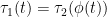
In calculus language, this would be a “re-parameterization” of a curve. If this happens, then the two curves that they describe coincide completely — they will overlap after a rotation and translation.

The above definition is derived from the plausible requirement for the following to hold:

$\int _{c}^d f(t) \ell _1(t) dt = \int _{\phi (c)}^{\phi (d)} f(s) \ell _2(s) ds, \ \forall [c, d]$

A change of variable $s=\phi (u)$ in the second integral leads to the first condition in the definition above.

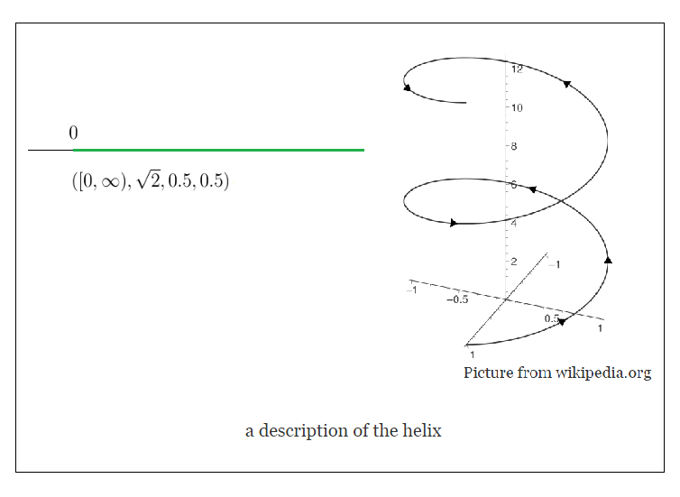
Image by Behnam Esmayli.

Example:

We saw from our previous example that $([0,1], \ \sqrt{1+4t^2}, \ 2(1+4t^2)^{-3/2}, 0)$ describes a part of the parabola $y=x^2$ .

It turns out that the set of data $([0,1], \ \sqrt{1+\frac {4}{s}}, \ 2(1+4s)^{-3/2}, \ 0)$ also describes the same curve, with an explicit equivalence being given by the map $s=t^2=\phi (t)$ .

Intrinsic Integration On Curves

Suppose that we are given a function which assigns to each point on a curve a real number, say the temperature at that point. We wish to find the average temperature over the curve. To do this, we need to add up (integrate) the temperatures at each point and divide the result by total number of points (length).

The following is an appropriate definition of the integral of a real-valued continuous function $f$ on our manifold:

$\int f := \int _{t_1}^{t_2} f(t) \ell (t) dt.$

Again, it is adding up values of $f$ on $I$ , just as in Riemann sum, except that now we have a non-uniform weight $\ell (t)$ applied to each summand.

The reason this definition works is that if we calculate the integral using a different but equivalent set of data, then by the change-of-variables formula, we would get the same answer:

$\int f := \int _{t_1}^{t_2} f(t) \ell (t) dt = \int _{s_1}^{s_2} f(s) \ell (s) ds.$

Observation: Our definition of integration only depended on the function $\ell$ . Therefore, it suffices to have a way of measuring distances in order to be able to define a parameterization-free, $\mathbb{R}^3$ -free notion of integration on a curve.

Note: The integration above may be familiar from calculus, or complex functions, as a “line integral”. But it is usually not emphasized there that this is intrinsic to the curve. However, it indeed comes with the curve, independent of the embedding of the curve in $\mathbb{R}^3.$

What’s next …

Now that we know a way of telling when two parameterizations coincide, in the next installment, we will be able to “glue together” pieces to arrive at a manifold.

The definition of the integration will work globally because different parameterizations agree on it locally.

What is a Manifold? (2/6)

About Behnam Esmayli

Categories

Archives

Retired Blogs

Meta